Position-Time Graphs
How motion becomes a picture, and why the slope hides the velocity
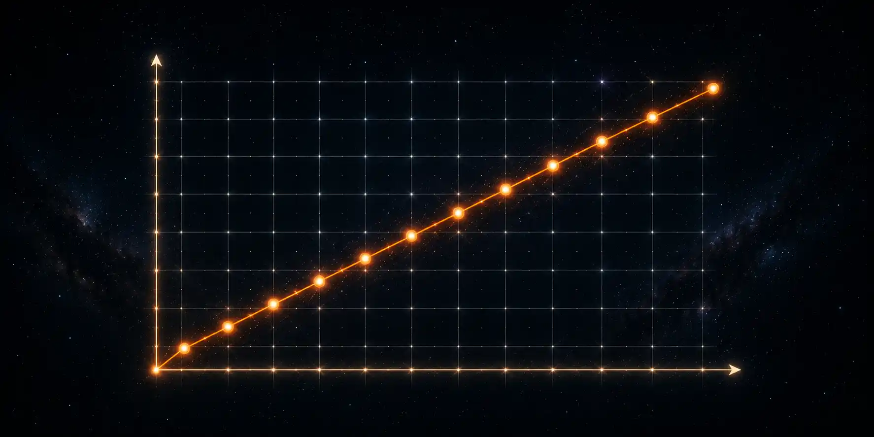
Imagine you ask your friend Riya to track her location every second as she walks from her house to school. She gives you a list of numbers: 0 m, 20 m, 40 m, 60 m, 80 m, 100 m, 120 m — one number per second.
If you draw these as dots on a graph with time on one axis and position on the other — what shape do you think the dots will make? What would that shape tell you about how she walked?
Each second she covers exactly the same extra distance — what kind of line connects equally spaced dots?
The Verse on Time as the Pattern Behind Everything
कालो ह भूतं भव्यं च पुत्रो अजनयत् पुरा ।
कालादृचः समभवन् यजुः कालादजायत ॥
"काल ही ने जो था, जो होगा — सब कुछ रचा है। उसी से ऋचाएँ निकलीं, उसी से यजुष् पैदा हुआ। काल हर चीज़ का साँचा है।"
"Time is the womb that bore the past and the future. From Time arose the verses; from Time arose the sacred chants. Time is the pattern beneath all things."
— The Kāla Sūkta of the Atharva Veda treats time itself as a thing worth studying — not just a backdrop, but a measurable, patterning force. The graph you will draw on this page does exactly what the sūkta points to: it reveals the pattern of motion across time. Plot position against time, and time becomes visible as a shape.
Why Graphs?
A table of numbers tells you the data. A graph tells you the story. Looking at in a column requires effort to read; the same numbers plotted as a straight line communicate "steady, even motion" in a single glance. The whole point of a graph is to compress many numbers into one shape your eye can read instantly. From this page onwards, almost every motion problem you meet can be solved by looking at the right graph.
Plotting a position-time graph
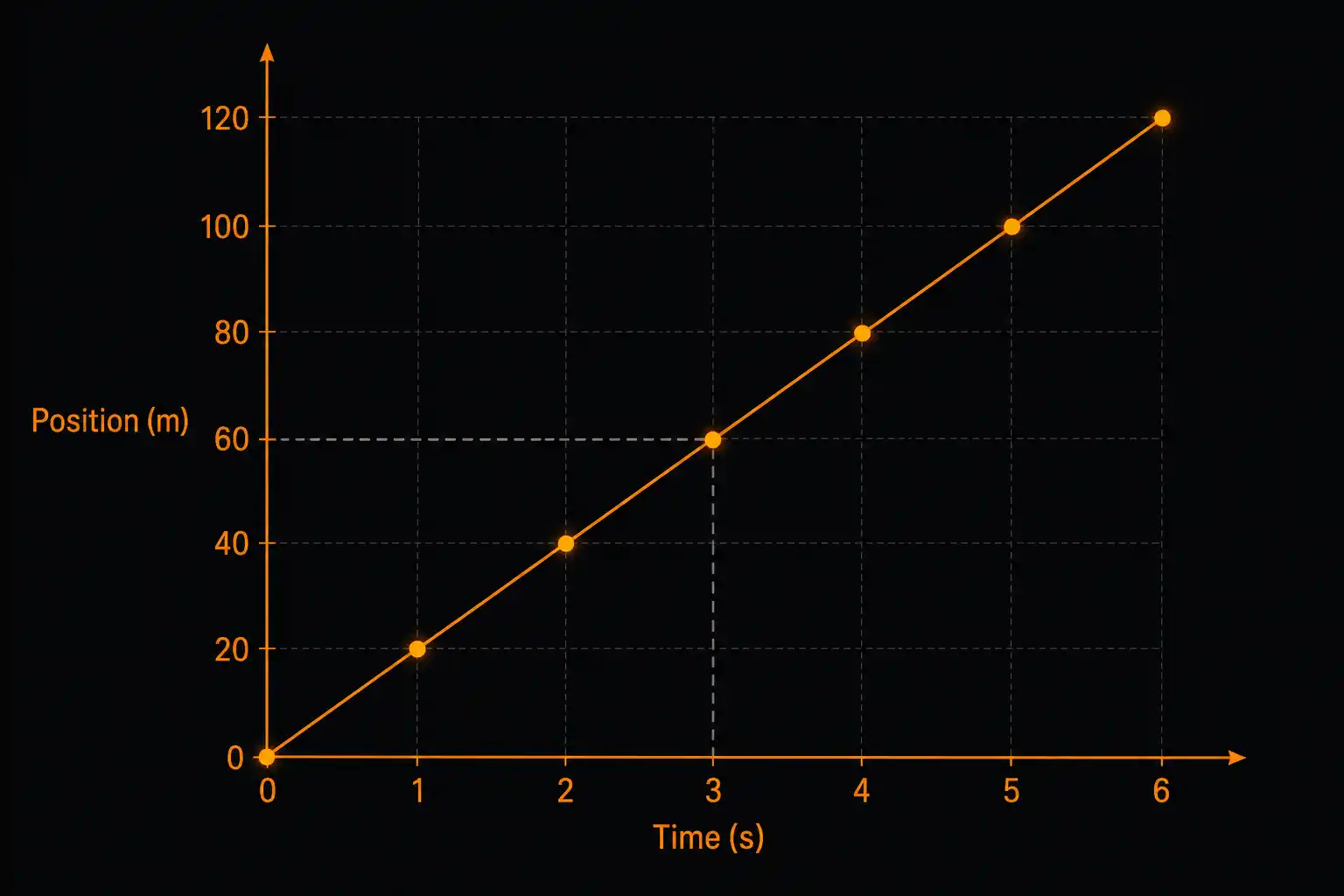
Suppose a vehicle is moving on a straight road and we record its position from a fixed origin at every second:
| Time (s) | 0 | 1 | 2 | 3 | 4 | 5 | 6 |
|---|---|---|---|---|---|---|---|
| Position (m) | 0 | 20 | 40 | 60 | 80 | 100 | 120 |
To turn this into a graph, follow four steps:
- Draw two perpendicular axes. The horizontal axis is the x-axis; the vertical axis is the y-axis. Their meeting point is the origin O.
- Decide which quantity goes on which axis. The convention for motion: time on the x-axis, position on the y-axis. (The independent variable — what you control — goes on the x-axis. You choose the times; you measure the positions.)
- Choose a scale that uses the available space. For our data, 5 small divisions = 1 second on the x-axis and 5 small divisions = 20 m on the y-axis works well — the graph fills the page without crowding.
- Plot each (time, position) pair as a single dot. For (1 s, 20 m), find the point that is 1 second along the x-axis and 20 m up the y-axis — and place a dot. Repeat for every row of the table.
When all dots are placed, join them with a single smooth line. That line is the position-time graph of the motion. For our data, the dots fall on a perfectly straight line — the signature of constant velocity, as we'll see in the next section.
What the shape tells you
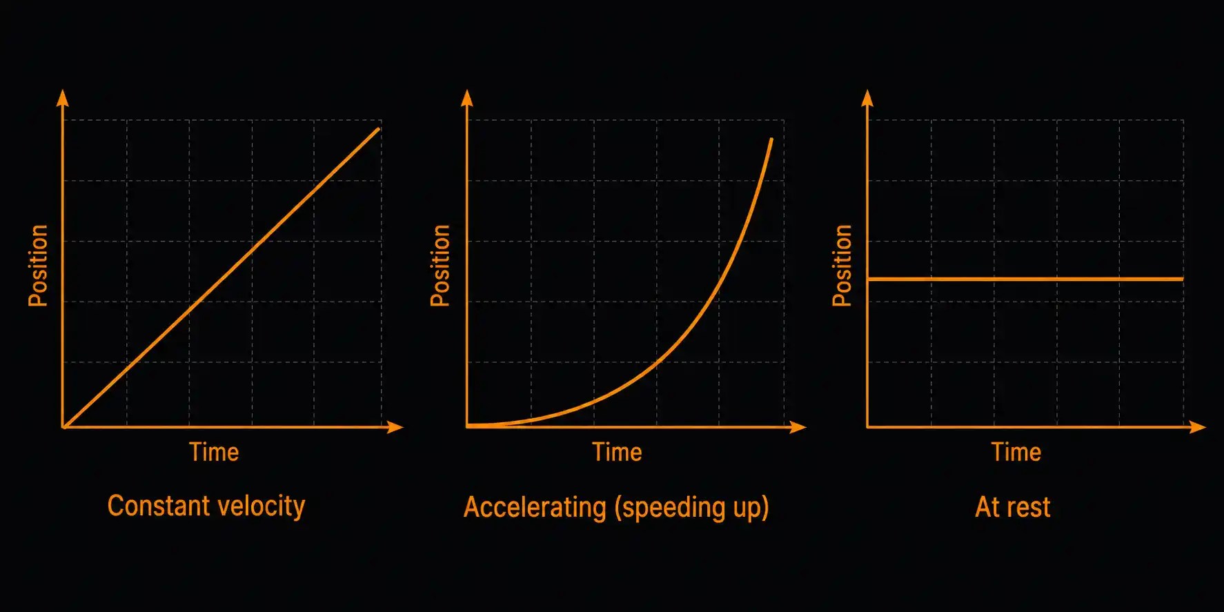
Once a position-time graph is drawn, you can read the kind of motion straight off the shape — without any calculation. There are three shapes you must recognise instantly:
1. Straight line (going up or down) → constant velocity.
If in equal time intervals the position changes by equal amounts, the dots line up perfectly. Every second, the same step. The slope (steepness) tells you the speed; the direction (rising or falling) tells you the sign of velocity.
2. Curved line → changing velocity → the object is accelerating.
If the position changes by unequal amounts in equal time intervals — small step at first, bigger steps later — the line bends. A curve that gets steeper means the object is speeding up. A curve that flattens means the object is slowing down.
3. Horizontal straight line → object is at rest.
If the position does not change with time, the dots all sit at the same height. The line is parallel to the x-axis. The object is parked.
Memorise these three shapes. They are the alphabet of motion graphs. Almost every position-time graph you will see in this book — and in every physics exam — is some combination of these three.
A caution: a position-time graph is not a route map. It does not show the path the object travelled along the road; it shows how its position (a single number on the chosen axis) changed with time. A bus driving north for an hour and a bus driving south for an hour can have position-time graphs that are mirror images, but they are not driving on the same road.
Slope of the line = velocity
The shape tells you what kind of motion. The slope tells you how fast.
The slope of any straight line is its steepness — how much it rises as you go across. On a position-time graph, slope is precisely:
But that is exactly the formula for average velocity! So:
The slope of the position-time graph at any segment is equal to the average velocity over that segment.
This is the single most important sentence on this page.
The triangle trick. To find the slope between two points and on the line, drop a horizontal line from rightward and a vertical line from downward. You get a right triangle with in the top-left, in the top-right, and in the bottom-right corner.
- The horizontal leg is the time interval .
- The vertical leg is the change in position .
- The slope is — and this number, in m/s, is the velocity.
A steep line means a large slope means a high velocity. A shallow line means a small slope means a low velocity. A horizontal line has slope zero — and zero velocity, which is the same as being at rest. Three shapes, one number to compute.
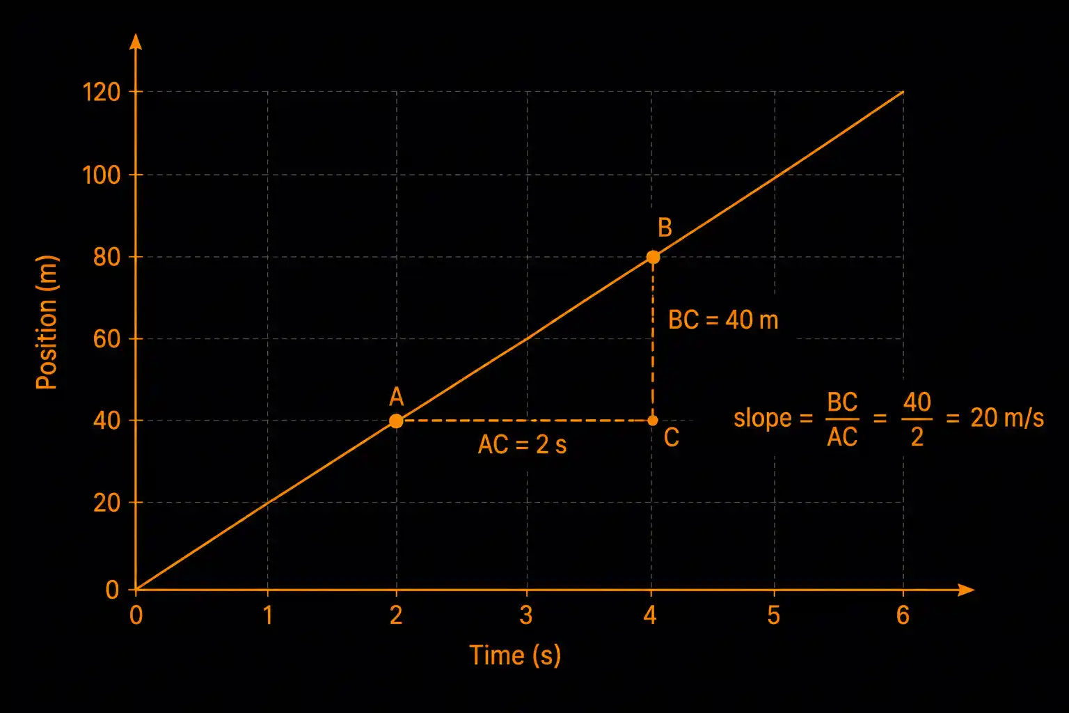
From the position-time graph above (a straight line passing through the origin and through (6 s, 120 m)), calculate the average velocity of the vehicle between and .
Loading simulator…
You are shown a position-time graph for two cars, A and B, both starting from the same position at . The line for car B is steeper than the line for car A throughout the graph.
Both lines are straight. Which conclusion is correct?
Threads of Curiosity — Graphs Are the Language Physics Speaks
Walk into any working physics lab — at the Indian Institute of Astrophysics in Bengaluru, at the Tata Institute in Mumbai, at the Inter-University Centre in Pune — and the walls will be covered in graphs. Earthquake plots. Stellar light curves. Particle detector traces. Voltage-time recordings. Graphs are the second language of every working scientist.
Q1.On a standard position-time graph, what is plotted on which axis?
Imagine you ask your friend Riya to track her location every second as she walks from her house to school. She gives you a list of numbers: 0 m, 20 m, 40 m, 60 m, 80 m, 100 m, 120 m — one number per second.
If you draw these as dots on a graph with time on one axis and position on the other — what shape do you think the dots will make? What would that shape tell you about how she walked?
Each second she covers exactly the same extra distance — what kind of line connects equally spaced dots?
The Verse on Time as the Pattern Behind Everything
कालो ह भूतं भव्यं च पुत्रो अजनयत् पुरा ।
कालादृचः समभवन् यजुः कालादजायत ॥
"काल ही ने जो था, जो होगा — सब कुछ रचा है। उसी से ऋचाएँ निकलीं, उसी से यजुष् पैदा हुआ। काल हर चीज़ का साँचा है।"
"Time is the womb that bore the past and the future. From Time arose the verses; from Time arose the sacred chants. Time is the pattern beneath all things."
— The Kāla Sūkta of the Atharva Veda treats time itself as a thing worth studying — not just a backdrop, but a measurable, patterning force. The graph you will draw on this page does exactly what the sūkta points to: it reveals the pattern of motion across time. Plot position against time, and time becomes visible as a shape.
Why Graphs?
A table of numbers tells you the data. A graph tells you the story. Looking at in a column requires effort to read; the same numbers plotted as a straight line communicate "steady, even motion" in a single glance. The whole point of a graph is to compress many numbers into one shape your eye can read instantly. From this page onwards, almost every motion problem you meet can be solved by looking at the right graph.
Plotting a position-time graph
Suppose a vehicle is moving on a straight road and we record its position from a fixed origin at every second:
| Time (s) | 0 | 1 | 2 | 3 | 4 | 5 | 6 |
|---|---|---|---|---|---|---|---|
| Position (m) | 0 | 20 | 40 | 60 | 80 | 100 | 120 |
To turn this into a graph, follow four steps:
- Draw two perpendicular axes. The horizontal axis is the x-axis; the vertical axis is the y-axis. Their meeting point is the origin O.
- Decide which quantity goes on which axis. The convention for motion: time on the x-axis, position on the y-axis. (The independent variable — what you control — goes on the x-axis. You choose the times; you measure the positions.)
- Choose a scale that uses the available space. For our data, 5 small divisions = 1 second on the x-axis and 5 small divisions = 20 m on the y-axis works well — the graph fills the page without crowding.
- Plot each (time, position) pair as a single dot. For (1 s, 20 m), find the point that is 1 second along the x-axis and 20 m up the y-axis — and place a dot. Repeat for every row of the table.
When all dots are placed, join them with a single smooth line. That line is the position-time graph of the motion. For our data, the dots fall on a perfectly straight line — the signature of constant velocity, as we'll see in the next section.
What the shape tells you
Once a position-time graph is drawn, you can read the kind of motion straight off the shape — without any calculation. There are three shapes you must recognise instantly:
1. Straight line (going up or down) → constant velocity.
If in equal time intervals the position changes by equal amounts, the dots line up perfectly. Every second, the same step. The slope (steepness) tells you the speed; the direction (rising or falling) tells you the sign of velocity.
2. Curved line → changing velocity → the object is accelerating.
If the position changes by unequal amounts in equal time intervals — small step at first, bigger steps later — the line bends. A curve that gets steeper means the object is speeding up. A curve that flattens means the object is slowing down.
3. Horizontal straight line → object is at rest.
If the position does not change with time, the dots all sit at the same height. The line is parallel to the x-axis. The object is parked.
Memorise these three shapes. They are the alphabet of motion graphs. Almost every position-time graph you will see in this book — and in every physics exam — is some combination of these three.
A caution: a position-time graph is not a route map. It does not show the path the object travelled along the road; it shows how its position (a single number on the chosen axis) changed with time. A bus driving north for an hour and a bus driving south for an hour can have position-time graphs that are mirror images, but they are not driving on the same road.
Slope of the line = velocity
The shape tells you what kind of motion. The slope tells you how fast.
The slope of any straight line is its steepness — how much it rises as you go across. On a position-time graph, slope is precisely:
But that is exactly the formula for average velocity! So:
The slope of the position-time graph at any segment is equal to the average velocity over that segment.
This is the single most important sentence on this page.
The triangle trick. To find the slope between two points and on the line, drop a horizontal line from rightward and a vertical line from downward. You get a right triangle with in the top-left, in the top-right, and in the bottom-right corner.
- The horizontal leg is the time interval .
- The vertical leg is the change in position .
- The slope is — and this number, in m/s, is the velocity.
A steep line means a large slope means a high velocity. A shallow line means a small slope means a low velocity. A horizontal line has slope zero — and zero velocity, which is the same as being at rest. Three shapes, one number to compute.
From the position-time graph above (a straight line passing through the origin and through (6 s, 120 m)), calculate the average velocity of the vehicle between and .
Loading simulator…
You are shown a position-time graph for two cars, A and B, both starting from the same position at . The line for car B is steeper than the line for car A throughout the graph.
Both lines are straight. Which conclusion is correct?
Threads of Curiosity — Graphs Are the Language Physics Speaks
Walk into any working physics lab — at the Indian Institute of Astrophysics in Bengaluru, at the Tata Institute in Mumbai, at the Inter-University Centre in Pune — and the walls will be covered in graphs. Earthquake plots. Stellar light curves. Particle detector traces. Voltage-time recordings. Graphs are the second language of every working scientist.
Q1.On a standard position-time graph, what is plotted on which axis?